As you know, linear regression is a basic method in statistical modeling and machine learning. It provides a simple yet powerful way to predict a continuous outcome variable based on one or more predictor variables.
The core idea behind linear regression is to model the relationship between the dependent (response) variable and one or more independent (predictor) variables by fitting a linear equation to observed data.
The general form of a linear regression model with one predictor is:
\[
Y=β0 +β1 X+ϵ
\] Here, \(Y\) represents the dependent variable, \(X\) is the independent variable, \(β0\) is the intercept, \(β1\) is the slope coefficient, and \(ϵ\) denotes the error term, capturing the deviation of the observed values from the line of best fit.
You can read this as “Y equals beta zero, plus beta one times X, plus error”.
In multiple linear regression, where we use more than one predictor, the equation expands to:
\[
Y=β 0 +β 1 X 1 +β 2 X 2 +...+β n X n +ϵ
\]
Each \(β\) (beta) coefficient represents the change in the dependent variable for a one-unit change in the corresponding independent variable, holding all other variables constant.
The process of “fitting” a linear model involves estimating the \(β\) coefficients that minimise the sum of squared residuals, where a residual is the difference between an observed value and the value predicted by our model.
78.2 Implementing linear regression in R
R provides robust functionality for linear regression analysis through functions like lm(), which is used to fit linear models.
We’ve covered much of this ground in earlier sections of the module, but here’s a step-by-step reminder on how to implement linear regression in R:
Data Preparation: Ensure the data is clean and formatted correctly. Numerical variables should be used for the regression, and categorical variables need to be encoded appropriately.
Model Fitting: Use the lm() function to fit a linear model. The basic syntax is lm(Y ~ X1 + X2 + ..., data = your_data), where Y is the dependent variable, and X1, X2, ... are the independent variables.
Model Checking: After fitting the model, check the model’s summary using summary(your_model). This summary provides important information, including the regression coefficients, standard errors, and p-values for each predictor.
Diagnostics: Conduct diagnostic checks to validate assumptions like linearity, independence, homoscedasticity, and normality of residuals. Plots like residual vs. fitted values or Q-Q plots can be very helpful.
Here’s a brief example in R:
# create a linear regression modelmodel <-lm(mpg ~ wt + hp, data = mtcars)summary(model)
Call:
lm(formula = mpg ~ wt + hp, data = mtcars)

Residuals:
   Min     1Q Median     3Q    Max
-3.941 -1.600 -0.182  1.050  5.854

Coefficients:
            Estimate Std. Error t value Pr(>|t|)
(Intercept) 37.22727    1.59879  23.285  < 2e-16 ***
wt          -3.87783    0.63273  -6.129 1.12e-06 ***
hp          -0.03177    0.00903  -3.519  0.00145 **
---
Signif. codes:  0 '***' 0.001 '**' 0.01 '*' 0.05 '.' 0.1 ' ' 1

Residual standard error: 2.593 on 29 degrees of freedom
Multiple R-squared:  0.8268,    Adjusted R-squared:  0.8148
F-statistic: 69.21 on 2 and 29 DF,  p-value: 9.109e-12
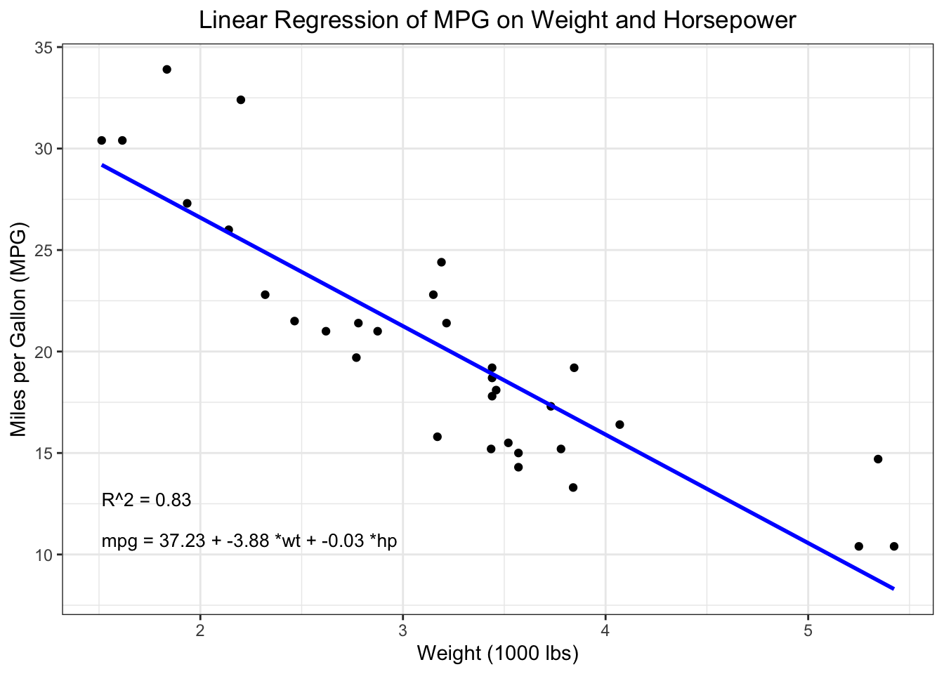
## create a visualisation# librarieslibrary(ggplot2)library(ggpmisc)# summary of the model to extract coefficients and R-squaredmodel_summary <-summary(model)equation <-paste("mpg =",format(round(model_summary$coefficients[1], 2), nsmall =2), "+",format(round(model_summary$coefficients[2], 2), nsmall =2), "*wt +",format(round(model_summary$coefficients[3], 2), nsmall =2), "*hp")r_squared <-paste("R^2 =", format(round(model_summary$r.squared, 2), nsmall =2))# Create plot, including regression equation annotated on plotp <-ggplot(mtcars, aes(x = wt, y = mpg)) +geom_point() +geom_smooth(method ="lm", formula = y ~ x, se =FALSE, color ="blue") +theme_minimal() +labs(title ="Linear Regression of MPG on Weight and Horsepower",x ="Weight (1000 lbs)",y ="Miles per Gallon (MPG)") +annotate("text", x =min(mtcars$wt), y =min(mtcars$mpg), label = equation, hjust =0, vjust =0, size =3.5) +annotate("text", x =min(mtcars$wt), y =min(mtcars$mpg) +2, label = r_squared, hjust =0, vjust =0, size =3.5) +theme_bw() +theme(plot.title =element_text(hjust =0.5))# Print plotprint(p)
78.3 Understanding model output and model fit
Understanding the output of a linear regression model is crucial for interpreting the results and assessing the model’s efficacy.
Key components of the model output include:
Coefficients: These values indicate the estimated change in the dependent variable for a one-unit change in the predictor variable. The intercept \((β0)\) represents the value of \(Y\) when all Xs are 0. In the model above the intercept = 37.23.
R-squared (R²): This statistic provides a measure of how well the observed outcomes are replicated by the model, based on the proportion of total variation of outcomes explained by the model. In the example above, R² = 0.83, suggesting around 83% of the total variance in the outcome (MPG) is explained by 37.23 + (-3.88 * wt) + (-0.03 * hp).
Adjusted R-squared: Particularly important in multiple regression, this adjusts the R² for the number of predictors in the model, providing a more accurate measure of model fit.
F-statistic: This tests the null hypothesis that all regression coefficients are equal to zero, essentially checking whether the model provides a betterfit than a model with no predictors.
p-values: These provide the probability of observing the data (or something more extreme) assuming that the null hypothesis is true. In the context of regression, a p-value for each coefficient tests the null hypothesis that the coefficient is zero.
Residual Standard Error (RSE): This reflects the average distance that the observed values fall from the regression line.
By examining these outputs, you can assess the reliability and predictive power of your linear regression model, and make further adjustments or interpretations in line with your objectives as an analyst.